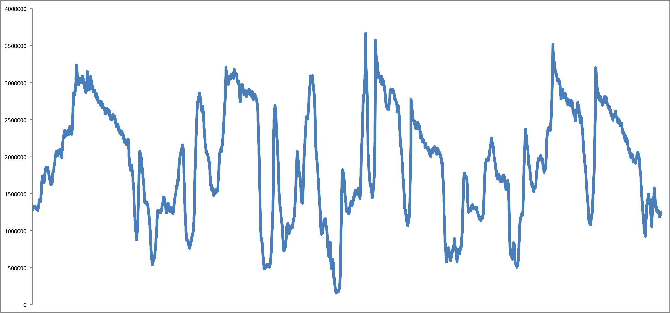
Four hundred thousand years is a difficult span to hold in your attention. In this series of compositions, changes in Antarctic ice become changes in rhythm, pitch, density, and texture. Deep time takes the length of a listening experience.
Created with Professor Mark Ballora and the Penn State Polar Center, the work uses the center's data on ice area and volume, floating ice, solar radiation, basal temperature, and sea level. I worked in SuperCollider to give those variables distinct sonic behaviors, composing an instrument system that the data could play.
Six voices for a changing continent.
The central design decision was to give the variables different timbral identities. A listener needs a way to stay with a variable as its values change and as other variables sound alongside it. Percussion, drones, noise, and granular tones offer different kinds of presence in the same composition.
Total ice volume drives a resonant percussion voice built from DynKlank, a bank of tuned resonators. Random impulses excite the instrument while the data changes its frequencies, trigger rates, spatial spread, and reverberation. A numerical change can therefore alter the character of an entire texture.
Grounded ice area and volume shape a low oscillator voice, with pitch and amplitude following the land-based ice. Floating ice uses filtered noise bursts. Their density and cutoff respond to the data, giving this part of the composition a granular, crackling quality.
Build relationships the ear can follow.
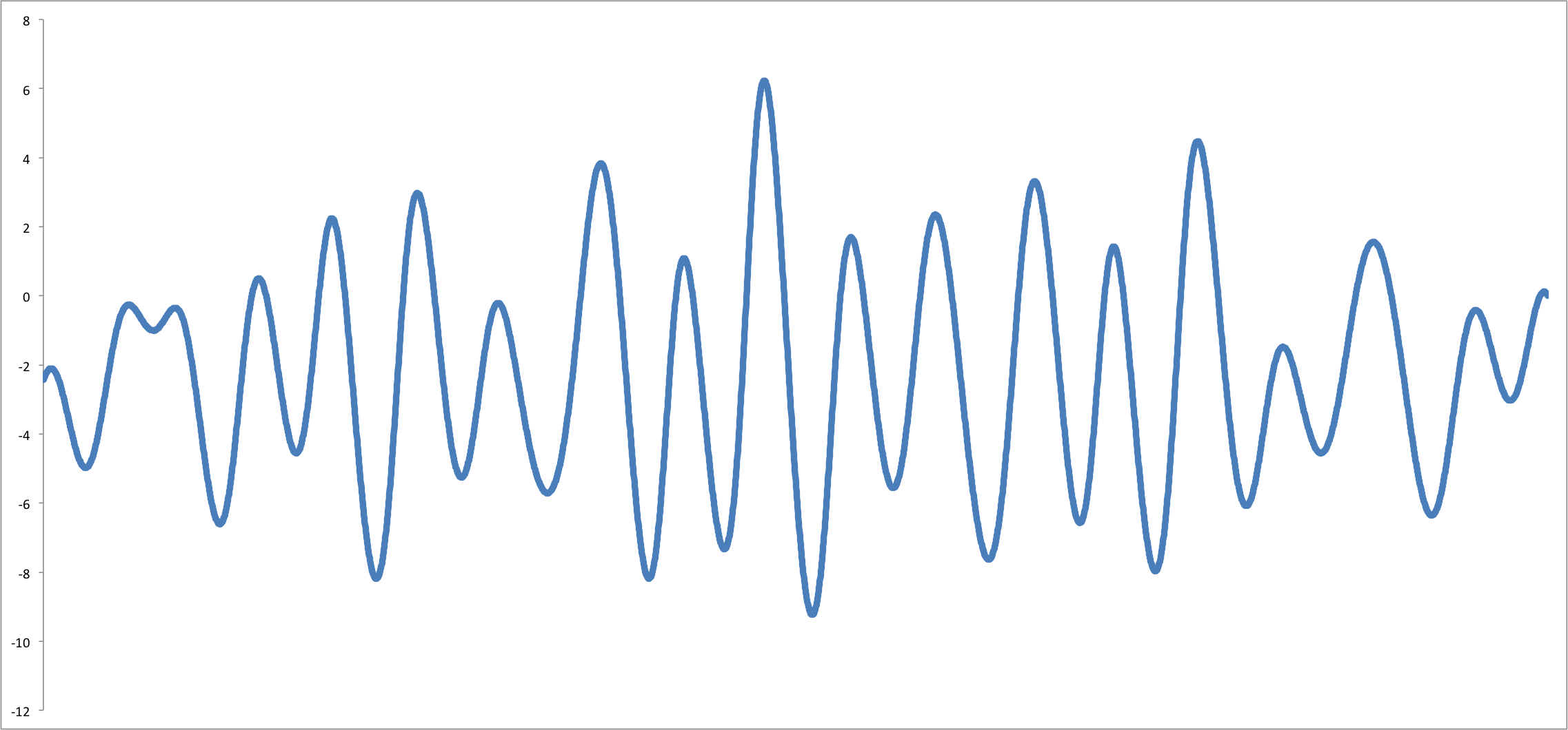
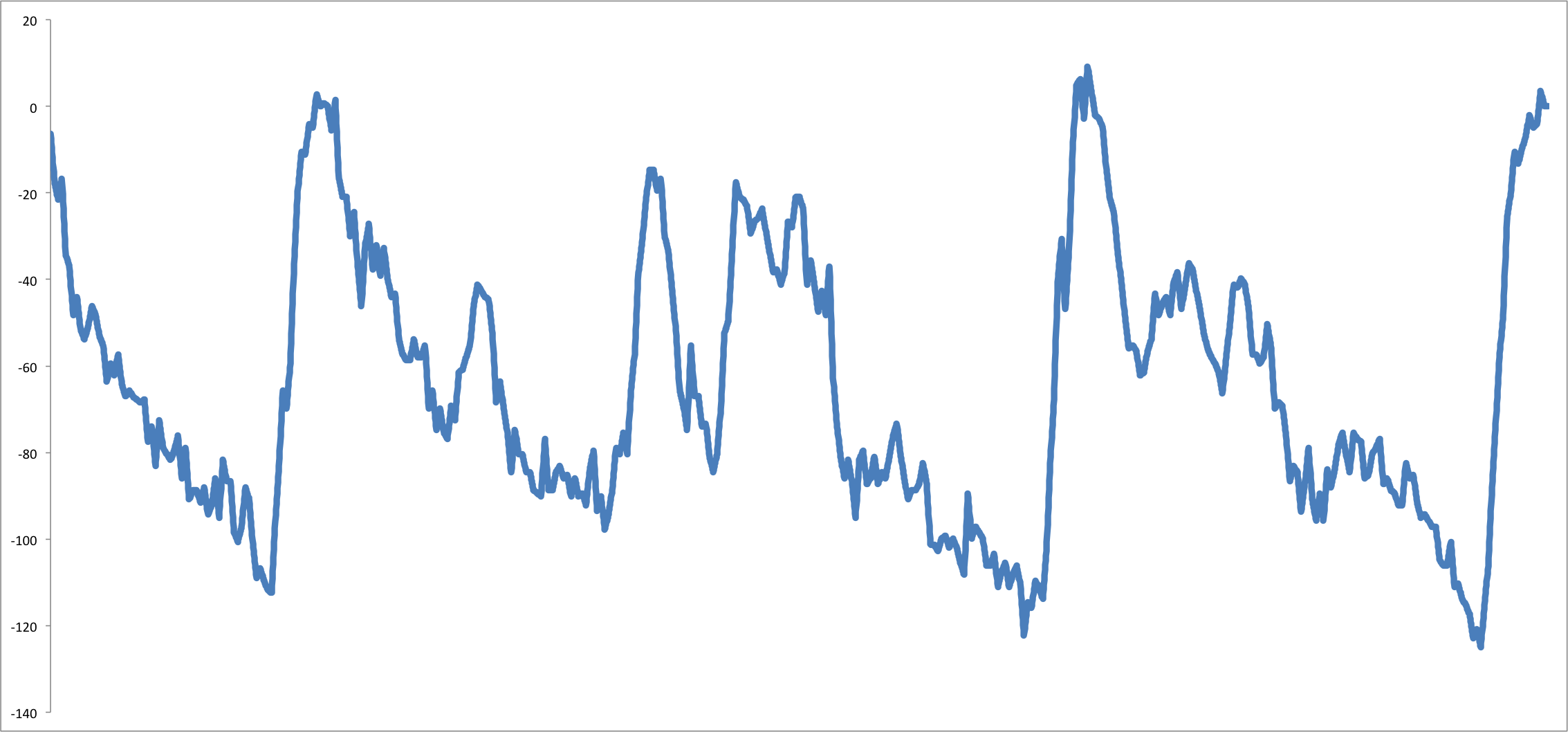
Sea level controls a water-like instrument made from filtered impulses. Pitch, event density, and stereo width change together. Solar radiation drives a granular FM voice with comb-filter delays, bringing a brighter sound into the field. Basal temperature shapes a more complex voice built from formant-filtered noise, resonant brown noise, and detuned sawtooth waves.
Each voice carries several audible dimensions. Loudness can change with a variable while its rhythm, register, or texture changes too. The composition can open out, gather density, or develop a different balance between its parts as the dataset advances.
Those mappings are compositional choices. The instruments establish how the values become perceptible; the data supplies their movement through time. Sound gives the relationships between variables a temporal form that can be followed as it unfolds.
A timescale you can listen through.
The series brings ice, ocean, sunlight, and temperature into one evolving field. Long cycles become phrases. Several variables can remain present at once, with changes appearing through their combination as well as through an individual voice.
The project sits where scientific representation becomes a listening practice. It asks for sustained attention to a system whose timescale is far outside ordinary experience, and gives that attention something concrete to follow: an event, a pulse, a texture that was there a moment ago and has now changed.
Inside the mapping.
The SuperCollider excerpt below sets up the data and normalizes its values into ranges for the instruments. It records the practical decisions behind the composition: how far a pitch can move, how dense a sequence can become, and how a measurement reaches a sound.
s.options.sampleRate = 48000;
s.reboot;
(
s.boot;
~buffer1=Buffer.alloc(s, 512, 1, {arg buf; buf.sine1Msg(1.0/[3, 4, 7, 8, 1, 2])});
~path="/Users/mbk5020/Desktop/SONIFICATION/polar day/polar iterations/";

~polardata=CSVFileReader.read(~path ++ "polardata.csv", true, true).asFloat;
~data=~polardata.flop;
///basaltemp
~basalTemperatures=thisProcess.interpreter.executeFile(~path ++ "basal_temp_info");
~basaltemps=Array.newClear(~basalTemperatures.size);
~basalTemperatures.do({ arg item, i; ~basaltemps.put(i, item[1]) });
~masterAmp=1;
)
////////////////////////////////////////////////////Data
(
~size=4001;
~timedelta=0.1;

~groundedIceArea = ~data.at(4).normalize(30, 90);
~groundedIceVolume = ~data.at(1).normalize(0, 0.2);

~floatingIceArea  = ~data.at(5).normalize(0, 1);
~floatingIceVolume = ~data.at(2).normalize(0.1, 6);
~floatingIceVLFP = ~data.at(2).normalize(1200, 1600);

~sealevel = ~data.at(7).normalize(1, 4);
~sealevelAmp = ~data.at(7).normalize(0.01, 1);

~trigrates=~data.at(3).normalize(7, 25);
~attacks=~data.at(3).normalize(0.02, 0.2);
~spreads=~data.at(3).normalize(0.25, 1);
~damps=~data.at(0).normalize(0.25, 1);
~roomsizes=~data.at(0).normalize(0.5, 0.7);
~freqscales=~data.at(0).reciprocal.normalize(0.5, 1.25);
~noiselevs=~data.at(0).normalize(0, 0.0025);
~levels=~data.at(0).normalize(0.5, 2);

~earthFundamental=7.83; // lowest Schumann resonance
~fund=~earthFundamental*32;
~sunPitches=~data.at(6).normalize(~fund*(5/6), ~fund*(6/5));
~sunCutoffs=~data.at(6).normalize(2500, 10000);
~sunDetunes=~data.at(6).normalize(-1, 5);

~groundarea=~data.at(4).normalize(60, 90);
~noiserqs=~data.at(4).normalize(0.005, 0.02);
~temperaturesSawVol=~basaltemps.normalize(0.01, 0.035);
~temperaturepitches=~basaltemps.normalize(30, 45);
~temperaturesSawDetunes=~basaltemps.normalize(0.1, 1);
~temperaturesSawCutoffs=~basaltemps.normalize(180, 1000);
)